Data Assimilation Project: Uncertainty-aware inference for complex dynamical systems
This project develops scalable methods for uncertainty quantification (UQ) and data assimilation (DA) in large dynamical systems. The emphasis is on combining ensemble-based and variational approaches with physics-informed statistical models (Gaussian processes) to enable robust state/parameter inference and uncertainty-aware prediction.
Scientific question
How do we infer hidden states and parameters from sparse noisy data?
Scientific DA problems combine partial observations, uncertain models, and large state spaces, so uncertainty has to be represented in a computationally realistic way.
Core idea
Combine numerical structure with statistical models
This work spans ensemble and variational DA, inverse problems, and physics-informed Gaussian processes, with each tool addressing a different computational bottleneck.
What visitors should learn
Different inference tasks need different approximations
The page is organized around four settings: chemistry DA, scalable 4D-Var, multi-output GP inference, and probabilistic climate forecasting.
Motivation
Many inference problems in science can be framed as estimating an evolving state $x(t)$ from partial and noisy observations $y(t)$, given an imperfect dynamical model. In discrete time, a common abstraction is
\[ x_{k+1} = \mathcal{M}_k(x_k) + \eta_k, \qquad y_k = \mathcal{H}_k(x_k) + \epsilon_k, \]
where $\mathcal{M}_k$ is the model propagator, $\mathcal{H}_k$ maps a model state to observation space, and $(\eta_k,\epsilon_k)$ represent model and observation errors. DA methods compute estimates of $x_k$ (and often uncertain parameters) while tracking uncertainty in a way that is accurate enough for decision support, but also computationally feasible at scale.
Ensemble and variational data assimilation: complementary tools
Two widely used paradigms are ensemble-based and variational data assimilation. They have different computational tradeoffs and failure modes, and many practical workflows mix ideas from both.
Variational DA (4D-Var)
4D-Var estimates an initial condition (and possibly parameters) by solving an optimization problem over an assimilation window:
\[ J(x_0) = \tfrac{1}{2}\lVert x_0 - x_b \rVert_{\mathbf{B}^{-1}}^2 \;+\; \tfrac{1}{2}\sum_{k=0}^{N} \lVert y_k - \mathcal{H}_k(\mathcal{M}_{0\to k}(x_0)) \rVert_{\mathbf{R}_k^{-1}}^2, \]
where $x_b$ is a background (prior) state, and $\mathbf{B},\mathbf{R}_k$ are background and observation error covariances. Gradients (and often Hessian-vector products) are computed with tangent-linear/adjoint models.
Ensemble Kalman methods (EnKF/EnKS)
Ensemble Kalman methods approximate uncertainty using an ensemble and apply Kalman-type updates at observation times. In a linearized form,
\[ x_k^{a} = x_k^{f} + \mathbf{K}_k \bigl(y_k - \mathbf{H}_k x_k^{f}\bigr), \qquad \mathbf{K}_k = \mathbf{P}_k^{f}\mathbf{H}_k^{T}\bigl(\mathbf{H}_k\mathbf{P}_k^{f}\mathbf{H}_k^{T} + \mathbf{R}_k \bigr)^{-1}, \]
with the forecast covariance $\mathbf{P}_k^{f}$ estimated from the ensemble.
Advantages and limitations
Ensemble methods: naturally parallel, no adjoint required, and provide sample-based uncertainty; but they suffer from sampling error in high dimension (spurious long-range correlations), often requiring localization and inflation, and they are sensitive to model error specification.
Variational methods: scale well with state dimension (no explicit covariance matrices) and can enforce model and constraint structure; but they require tangent-linear/adjoint capabilities and robust optimization, and they can be sensitive to nonconvexity and poor preconditioning.
What this project contributes
- Flow-dependent prior/error models for ensemble-based chemistry DA, including autoregressive (AR) background covariance construction and analysis of ensemble size/localization effects.
- Scalable variational DA strategies (low-memory smoothing and space-time domain decomposition) for large inverse problems.
- Physics-informed covariance modeling for multi-output Gaussian processes and hidden-process inference.
- Probabilistic GP forecasting workflows with explicit uncertainty calibration for time-series prediction problems.
Topic 1: Chemical data assimilation with EnKF and flow-dependent priors
Atmospheric chemistry DA is challenging because (i) the state is large and coupled across species, (ii) observations are sparse/heterogeneous, and (iii) background error structure is strongly flow-dependent. In ensemble Kalman workflows, the background covariance plays a central role because it controls how observation increments propagate through the model state.
One approach developed in this work models the background covariance through an autoregressive (AR) structure that captures distance decay and flow dependence. A representative construction is
\[ \mathbf{B} = \mathbf{A}^{-1}\mathbf{S}^2\mathbf{A}^{-T}, \qquad \delta c^{\mathrm{B}}(e) = \mathbf{A}^{-1}\mathbf{S}\,\xi(e), \qquad \xi(e)\sim \mathcal{N}(0,\mathbf{I}), \]
where $\mathbf{S}$ encodes spatially varying standard deviations and $\mathbf{A}$ encodes correlations (parameterized through an AR process). This provides a computationally practical way to inject physically meaningful structure into ensemble initialization and into the implied background statistics.
In addition, the chemistry DA studies in this project analyze sensitivity to practical algorithmic choices (ensemble size, localization/inflation strength, and error sources such as emissions and boundary conditions) and explore the use of model singular vectors as physically motivated perturbation directions for ensemble generation.
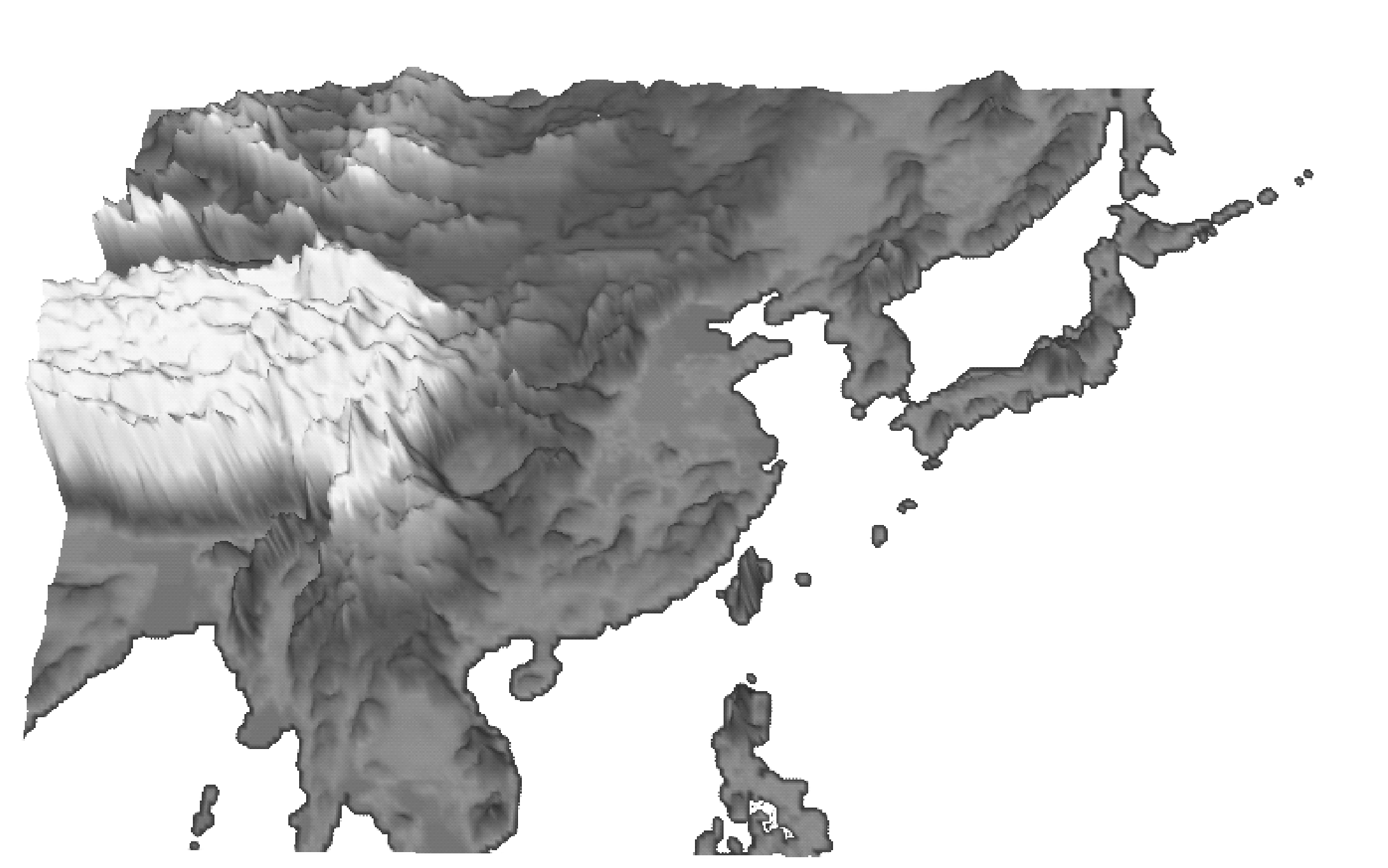
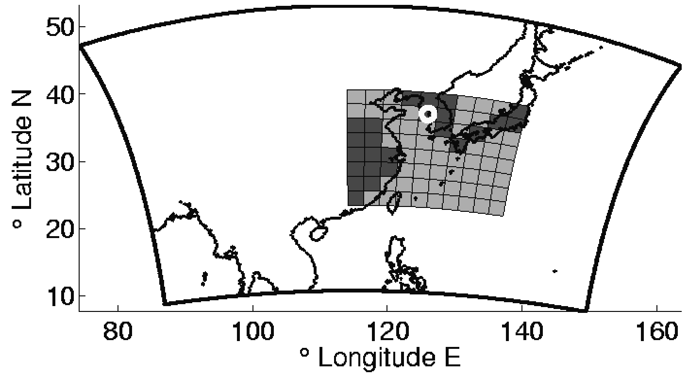
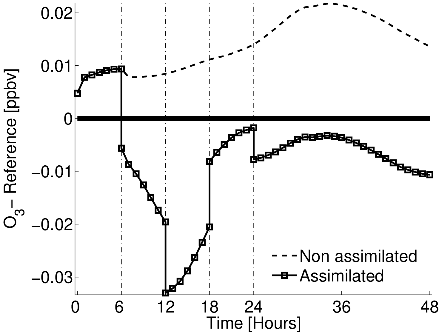
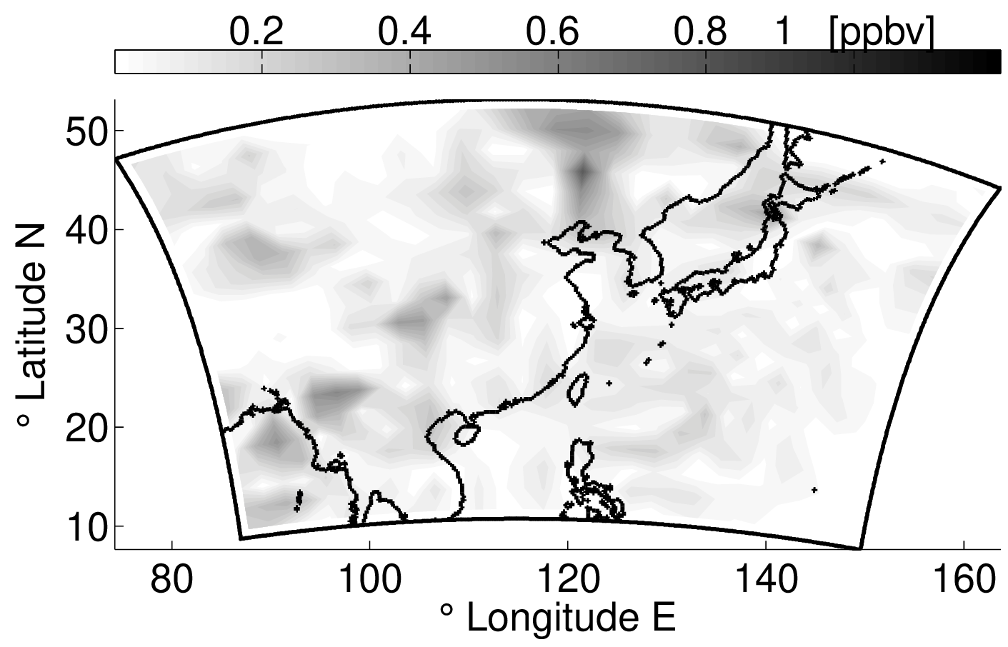
Chemistry DA: domain, observations, and forecast impact
Examples from an idealized chemistry transport model study: the domain and observation network, and a representative forecast improvement signal after assimilation.
Advantages and limitations
Advantages: AR-style priors provide a compact, flow-aware covariance structure that improves ensemble realism and can reduce spurious long-range correlations.
Limitations: covariance modeling is still approximate (especially under strong nonlinearity), and practical EnKF deployments still require careful tuning of localization, inflation, and model error representation.
Selected references
- Emil M Constantinescu, Adrian Sandu, Tianfeng Chai, and Gregory R. Carmichael. Assessment of ensemble-based chemical data assimilation in an idealized setting. Atmospheric Environment, Vol. 41(1); Pages 18-36, 2007. [DOI]
- Emil M Constantinescu, Tianfeng Chai, Adrian Sandu, and Gregory R. Carmichael. Autoregressive models of background errors for chemical data assimilation. Journal of Geophysical Research, Vol. 112; Pages D12309, 2007. [DOI]
- Adrian Sandu, Emil M Constantinescu, Gregory R. Carmichael, Tianfeng Chai, Dacian Daescu and John Seinfeld. Ensemble methods for dynamic data assimilation of chemical observations in atmospheric models. Journal of Algorithms & Computational Technology, Vol. 5(4); Pages 667-692, 2011.
Topic 2: Variational DA and scalable PDE-constrained inverse problems
In variational DA, the dominant cost often comes from repeatedly solving large linear/nonlinear systems inside an optimization method. This motivates algorithms that reduce memory footprint and expose parallel structure in space and time.
Two representative directions in this project are:
- Low-memory best-state estimation for hidden Markov models with model error, which targets large-scale inference where naive smoothing formulations become memory-prohibitive.
- Space-time domain decomposition for 4D-Var, which decomposes the inference problem into coupled local subproblems, enabling scalable solvers for large regularized inverse problems.
Scalable variational DA: local solvers and domain decomposition
These two images summarize the algorithmic theme in this part of the project: break a large inverse problem into computational units that are easier to solve and coordinate.


Advantages and limitations
Advantages: variational formulations provide a principled way to incorporate dynamical constraints and correlated error models, while domain decomposition can expose parallelism and reduce memory pressure.
Limitations: performance hinges on high-quality linear/nonlinear solvers and preconditioners; strong nonlinearity can lead to nonconvex optimization, and adjoint/tangent-linear infrastructure remains a key requirement.
Selected references
- Luisa D'amore, Emil M Constantinescu, and Luisa Carracciuolo. A scalable space-time domain decomposition approach for solving large scale non linear regularized inverse ill posed problems in 4D variational data assimilation,. Springer Journal of Scientific Computing, 2022. [DOI]
- Mihai Anitescu, Xiaoyan Zeng, and Emil M Constantinescu. A low-memory approach for best-state estimation of hidden Markov models with model error. SIAM Journal on Numerical Analysis (SINUM), Vol. 52(1); Pages 468-495, 2014. [DOI]
- Lin Zhang, Emil M Constantinescu, Adrian Sandu, Youhua Tang, Tianfeng Chai, Gregory R. Carmichael, Daewon Byun, and Eduardo Olaguer. An adjoint sensitivity analysis and 4D-Var data assimilation study of Texas air quality,. Atmospheric Environment (special ACM issue), Vol. 42(23); Pages 5787 - 5804, 2008. [DOI]
Topic 3: Physics-informed Gaussian processes for multi-output inference
Gaussian processes (GPs) provide a flexible, nonparametric route to inference with uncertainty quantification. A key practical challenge is specifying covariance structure that is both expressive and physically meaningful, especially for multiple outputs (co-kriging) and for settings where some processes are hidden/unobserved.
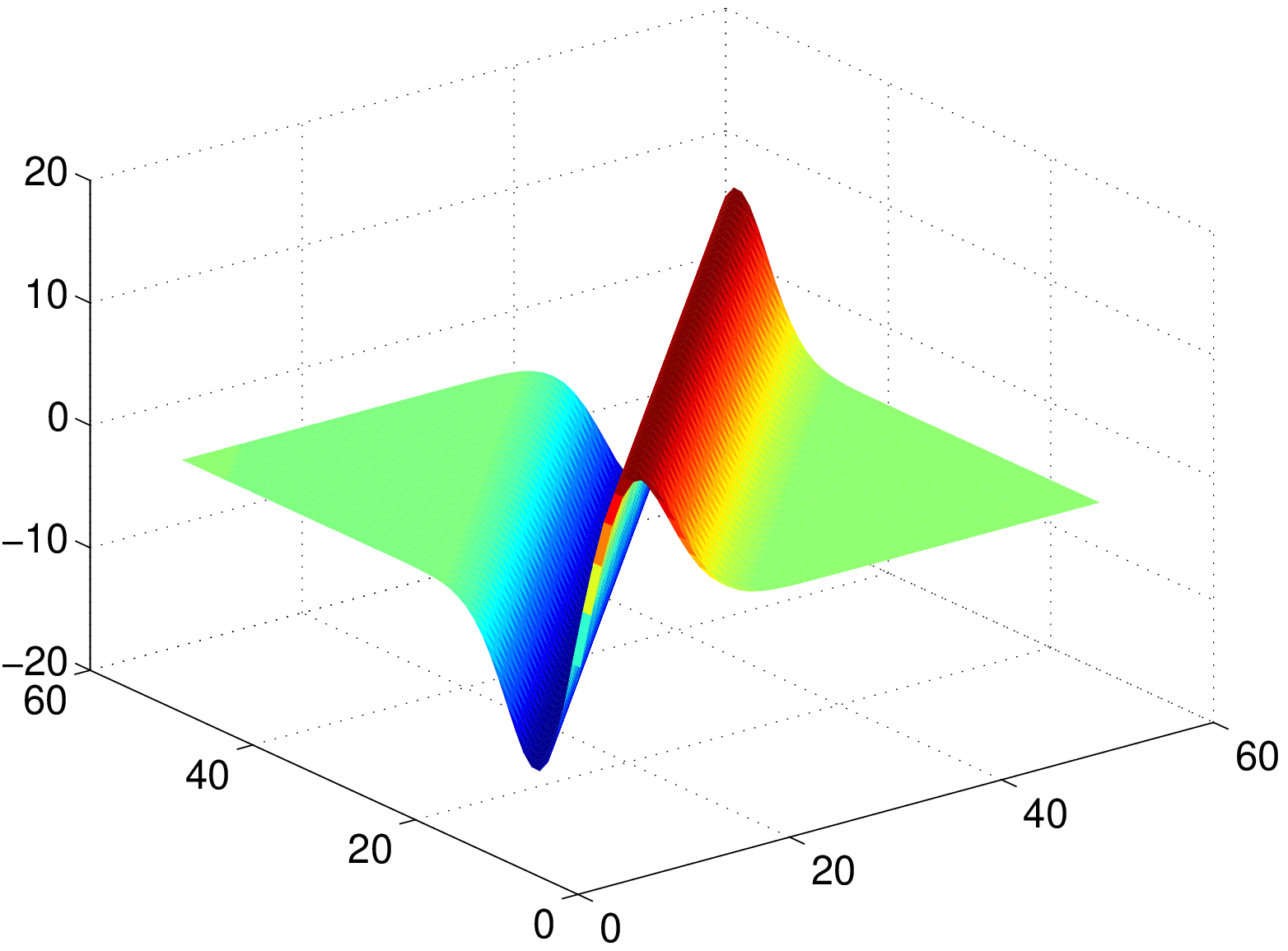
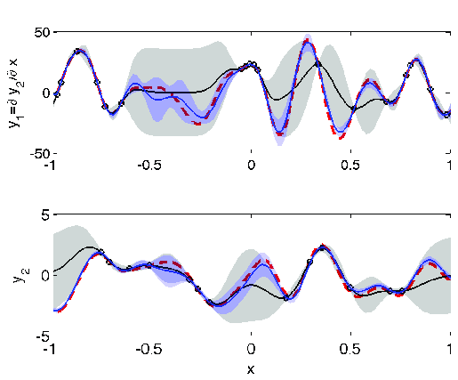
A physics-informed approach is to define outputs through linear operators acting on a latent GP $f$. If $y_i(x) = \mathcal{L}_i f(x)$ and $f \sim \mathcal{GP}(0,k)$, then the induced cross-covariance is
\[ \mathrm{Cov}\bigl(y_i(x),y_j(x')\bigr) = (\mathcal{L}_i)_x\,(\mathcal{L}_j)_{x'}\,k(x,x'). \]
This construction preserves positive definiteness by design, while enabling covariance models that reflect physical constraints (for example, relationships between pressure and wind derived from geostrophic assumptions).
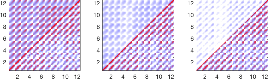
In space-time settings, GP models can also fuse deterministic numerical weather prediction (NWP) output with historical measurements to produce probabilistic forecasts and realistic scenario ensembles (with calibrated correlation structure).
Physics-informed covariance structure for multi-output GPs
The figures below move from model ingredient to model behavior: first a physics-induced cross-covariance surface, then a coupled multi-output regression example, and finally a wider space-time correlation comparison for wind scenario generation.
Advantages and limitations
Advantages: operator-based covariance construction is interpretable and embeds physical structure directly into the statistical model.
Limitations: when relationships among outputs are strongly nonlinear, additional closure assumptions may be needed; and scalable GP inference may require approximations for large datasets.
Selected references
- Emil M Constantinescu and Mihai Anitescu. Physics-based covariance models for Gaussian processes with multiple outputs. International Journal for Uncertainty Quantification, Vol. 3(1); Pages 47-71, 2013. [DOI]
- Julie Bessac, Emil M Constantinescu, and Mihai Anitescu. Stochastic simulation of predictive space-time scenarios of wind speed using observations and physical models. Annals of Applied Statistics, Vol. 12(1); Pages 432-458, 2018. [DOI] [arXiv]
Topic 4: Data-driven prediction with Gaussian processes (MJO forecasting)
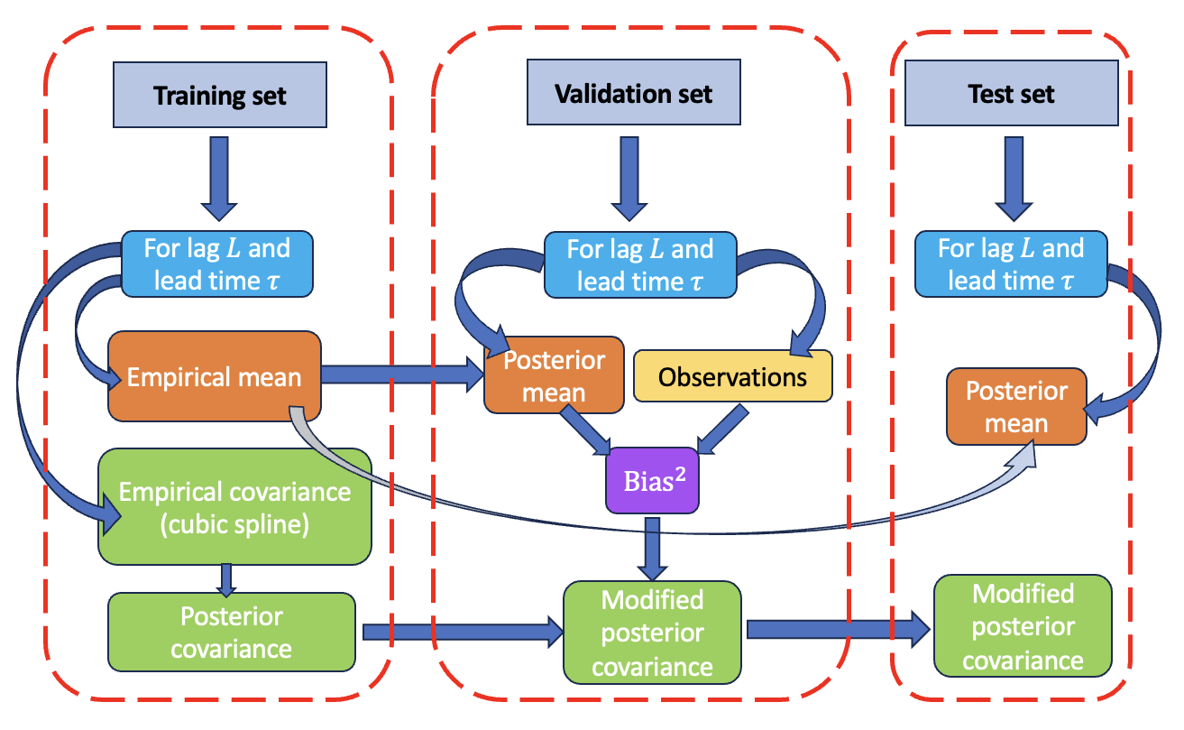
Recent work also explores GP models as a data-driven route to probabilistic forecasting of climate variability. For the Madden–Julian Oscillation (MJO), GP models can be calibrated using empirical correlations and then corrected a posteriori to better match forecast uncertainty. This yields both point forecasts and confidence intervals and enables diagnostic analysis of when uncertainty estimates are overconfident or miscalibrated.
In numerical experiments, this strategy improves deterministic prediction skill at short lead times and (through posterior covariance correction) substantially extends probabilistic coverage.
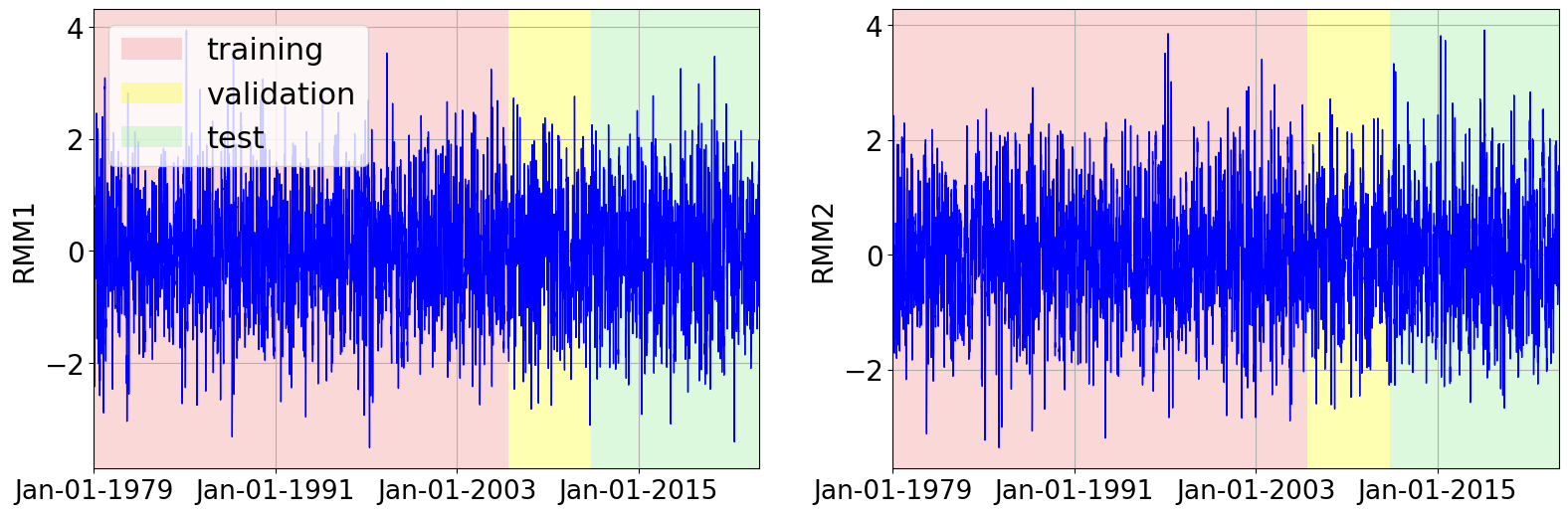
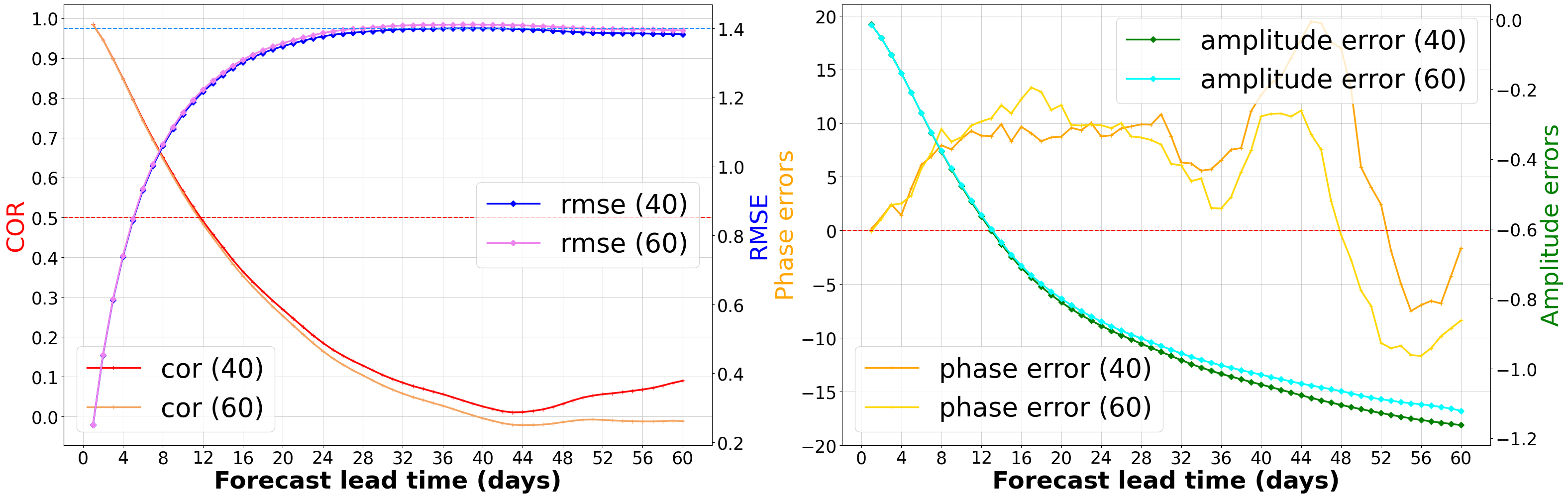
Gaussian process forecasting workflow (MJO)
These panels summarize three parts of the workflow: how the GP is calibrated and variance-corrected, how the RMM dataset is split into train/validation/test periods, and how deterministic and probabilistic forecast quality evolve with lead time.
Advantages and limitations
Advantages: GP forecasts are probabilistic by construction and provide uncertainty estimates that can be analyzed and corrected, rather than being purely heuristic.
Limitations: model calibration is sensitive to covariance structure choices and stationarity assumptions; scaling to very large datasets may require sparse/approximate GP techniques.
Selected references
- Haoyuan Chen, Emil M Constantinescu, Vishwas Rao, and Cristiana Stan. Improving the predictability of the Madden-Julian oscillation at subseasonal scales with Gaussian process models. JAMES - Machine learning application to Earth system modeling, Vol. 17(5); Pages e2023MS004188, 2025. [DOI] [arXiv]
- Haoyuan Chen, Emil M Constantinescu, Vishwas Rao, and Cristiana Stan. Uncertainty quantification of the Madden-Julian oscillation with Gaussian processes. 2023 Tackling Climate Change with Machine Learning Workshop, part of the 37th Conference on Neural Information Processing Systems (NeurIPS), 2023.
Software
Several of the methods above are implemented and tested in production-grade scientific computing libraries.
DAPack
Data assimilation toolkit
Research code for UQ/DA workflows and inverse problems.
PETSc TAO / TSAdjoint
Scalable optimization + adjoints
Nonlinear optimization and adjoint sensitivity analysis used in variational DA and PDE-constrained inversion.
Related pages
Funding
- U.S. Department of Energy, Office of Science, Office of Advanced Scientific Computing Research (ASCR) (including SciDAC programs on recent work).
- Argonne National Laboratory Directed Research and Development (LDRD) (on recent work).
- U.S. National Science Foundation, NOAA, and the Houston Advanced Research Center (on earlier chemistry DA work).