SciML Project: Disentangled latent spaces

This project develops interpretable generative models whose latent coordinates align with known physical drivers while preserving residual variability needed for realistic scientific data. The same latent-space design appears in three successive developments: Aux-VAE for representation learning, DL-CFM for higher-fidelity scientific generation, and disentangled deep priors for Bayesian inverse problems.

Thrust: Scientific machine learning Core idea: Guided and residual latent blocks Applications: Scientific generative modeling, cosmology, inverse problems

Scientific question

Can latent spaces reflect named physical factors?

Scientific datasets often come with some meaningful covariates, but not a complete factorization of all variability. The challenge is to align what is known without destroying generative flexibility.

Core idea

Split the latent space into guided and residual coordinates

A small latent block is softly tethered to auxiliary variables, while the remaining coordinates capture unresolved or unknown structure. This gives controllability without requiring full supervision.

Chronological thread

One design pattern, three increasingly ambitious uses

The project begins with disentangled representation learning, extends the same structure to higher-fidelity flow-based generation, and finally turns it into a prior for inverse problems.

Motivation

Many scientific datasets contain a mix of known and unknown sources of variation. Some physical quantities are measured or inferred and should have an interpretable role in the representation, while other mechanisms remain unmodeled or only partially understood. Standard deep generative models often compress these effects into entangled latent coordinates, which makes sensitivity analysis, controlled generation, and posterior interpretation harder than necessary.

This project studies a simple but powerful alternative: guide part of the latent space with auxiliary variables and reserve the rest for residual variability. That structure is useful not only for better representation learning, but also for anomaly discovery, interpretable scientific generation, and uncertainty-aware inverse problems.

Basic idea: disentangled latent spaces

Across the three developments, the common latent parameterization is

\[ z = \bigl(z_{\mathrm{aux}}, z_{\mathrm{rec}}\bigr), \qquad z_{\mathrm{aux}} \mid u \sim \mathcal{N}(u, \tau^2 I), \qquad z_{\mathrm{rec}} \sim \mathcal{N}(0, I), \qquad x = G_{\theta}(z_{\mathrm{aux}}, z_{\mathrm{rec}}). \]

Here $u$ denotes auxiliary variables with direct scientific meaning. The guided block $z_{\mathrm{aux}}$ is encouraged to align with those variables, while the residual block $z_{\mathrm{rec}}$ captures remaining variation that should not be forced into a named coordinate. In practical terms, this makes the latent space more useful for controlled traversals, response studies, outlier detection, and Bayesian posterior summaries.

What disentanglement means in this project

Interpretability: changing one guided coordinate should correspond to one physical effect rather than a mixture of unrelated changes.

Flexibility: the residual block should still absorb unresolved structure, so the model does not become brittle or over-constrained.

Transferability: the same split should remain useful when moving from representation learning to flow-based generation and then to inverse problems.

Development 1: Aux-VAE

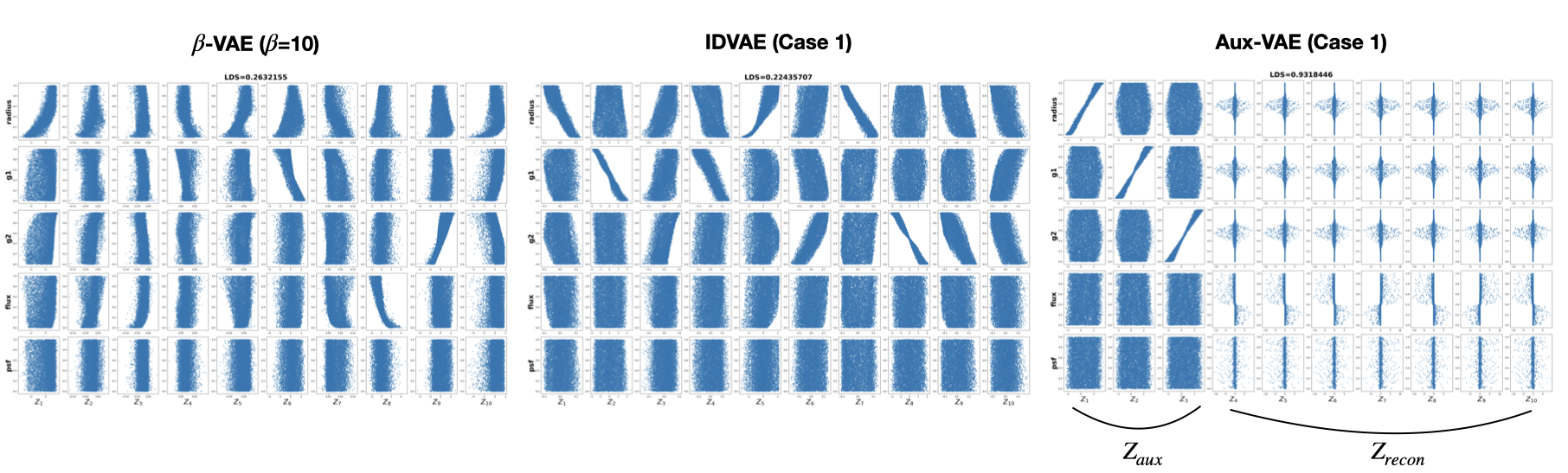
The first step is Aux-VAE, which introduces the guided/residual split inside a variational autoencoder. The model uses a conditional prior together with lightweight alignment and decorrelation penalties so that the first latent coordinates track the chosen auxiliary variables, while the remaining coordinates preserve reconstruction quality by representing unmodeled variability.

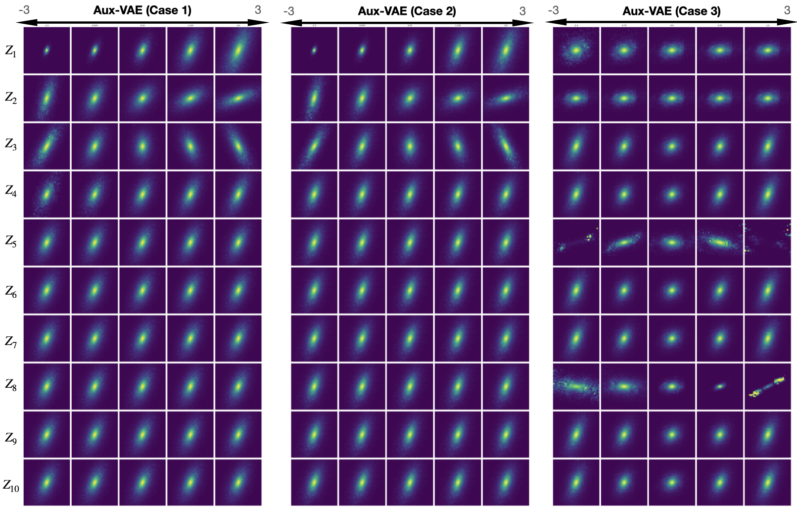
This matters because it keeps the architecture close to a standard VAE while making the latent space scientifically actionable. Instead of only asking whether the model reconstructs well, Aux-VAE asks whether the representation can be traversed and interpreted in terms of known generative factors. In the scientific-image experiments, this leads to clearer correspondence between selected latent coordinates and physically meaningful inputs.

Aux-VAE: interpretable traversal and factor alignment

The first figure shows that changing selected latent coordinates produces structured changes in the generated images. The second shows the intended one-to-one relationship between auxiliary variables and the first latent coordinates.

Latent traversal for Aux-VAE on the scientific image dataset — Aux-VAE latent traversals across several experimental cases. The guided block adapts to the auxiliary variables, while the residual block preserves the remaining reconstruction degrees of freedom.

Scatter plots between auxiliary variables and learned Aux-VAE latent coordinates — Scatter plots between auxiliary variables and learned latent coordinates. The goal is not full factorization of all variability, but a clean alignment of the selected coordinates with the known generating factors.

Development 2: DL-CFM

The second step, Disentangled Latent Conditional Flow Matching (DL-CFM), keeps the same latent-space idea but replaces the VAE-style generator with a more expressive flow-matching model. This addresses an important limitation of plain VAEs in scientific imaging: they can learn interpretable embeddings, but often smooth out fine structure and under-represent realistic sample variability.

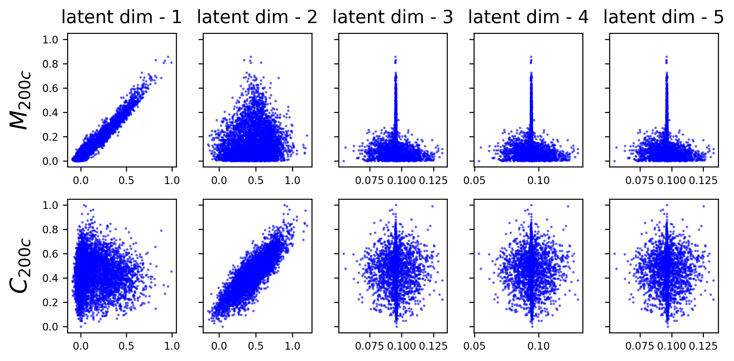
In the dark-matter halo application, the guided variables are halo mass and concentration derived from thermal Sunyaev-Zel’dovich maps. The first two latent coordinates are softly aligned with those quantities, while the residual coordinates capture remaining morphology. That makes the latent space useful for both controlled generation and diagnostics: one can move along physically meaningful axes while also probing residual-latent tails to surface unusual halo structure and candidate outliers.

DL-CFM: physical control with higher-fidelity generation

These figures illustrate the two roles of the latent split in DL-CFM: the guided coordinates track halo mass and concentration, while the residual coordinates expose structural variability beyond those named factors.

Guided DL-CFM latent coordinates aligned with halo mass and concentration — Alignment of guided latents with halo mass and concentration in DL-CFM. The goal is an interpretable low-dimensional control space, not just a compressed code.

Dark matter halo samples from residual-latent tails in DL-CFM — Samples generated from the tail of the reconstruction-focused latent block with the guided coordinates held fixed. This helps isolate unusual morphology and supports anomaly-style diagnostics.

Development 3: Disentangled deep priors for inverse problems

The third development takes the same latent decomposition and uses it as a structured prior for Bayesian inverse problems. Here the point is no longer only generation or traversal: the guided coordinates become named uncertain parameters, while the residual block carries unresolved field variability. This turns disentanglement into a prior-design principle for inference.

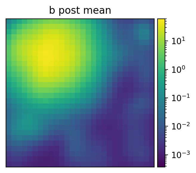
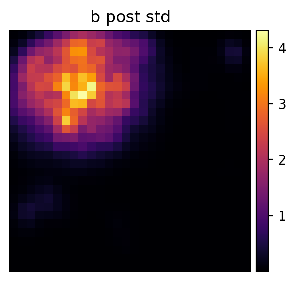
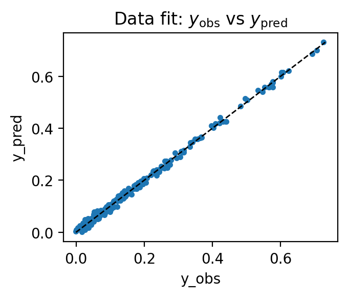
In elliptic PDE inverse problems, the resulting prior supports latent-space MAP estimation and MCMC sampling while keeping posterior summaries interpretable. Instead of a purely black-box generative prior, the posterior can be read in two layers: uncertainty in the physically meaningful auxiliary variables and uncertainty in the residual latent field. That is useful when the goal is not merely to fit observations, but to recover a scientifically meaningful uncertainty decomposition.

Deep priors: interpretable posteriors for inverse problems

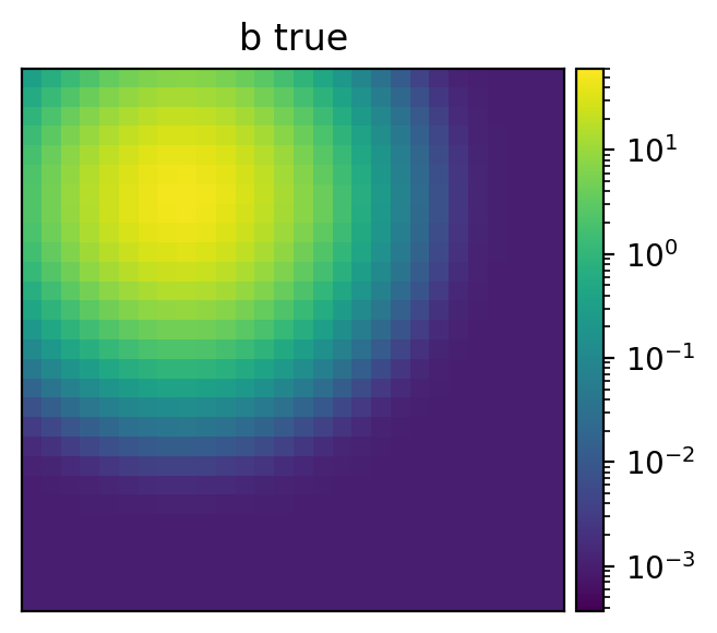
Representative source-identification results from an elliptic PDE inverse problem. The guided coordinates parameterize the dominant source characteristics, while the residual latent block captures remaining uncertainty in the reconstructed field.

Ground-truth source field for the inverse-problem example — Ground-truth source field used in the inverse-problem study.

Posterior mean field from the disentangled deep prior — Posterior mean field recovered with the disentangled deep prior.

Posterior standard deviation field from the disentangled deep prior — Posterior standard deviation, showing where uncertainty remains concentrated after assimilation of the observations.

Observed-versus-predicted data fit for the disentangled deep prior — Observed-versus-predicted data fit. The latent prior is designed to preserve interpretability without sacrificing the ability to match measurements.

References for deeper dive

Arkaprabha Ganguli, Nesar Ramachandra, Julie Bessac, and Emil M Constantinescu. Enhancing interpretability in generative modeling: Statistically disentangled latent spaces guided by generative factors in scientific datasets. Springer Machine Learning, Vol. 114(9); Pages 197, 2025. [DOI] [arXiv]
Arkaprabha Ganguli, Anirban Samaddar, Florian Kéruzoré, Nesar Ramachandra, Julie Bessac, Sandeep Madireddy, and Emil M Constantinescu. Uncovering physical drivers of dark matter halo structures with auxiliary-variable-guided generative models. Submitted, 2026. [arXiv] [PDF]
Arkaprabha Ganguli and Emil M Constantinescu. Disentangled deep priors for Bayesian inverse problems. Submitted, 2026. [arXiv] [PDF]