SciML Project: Hybrid ML-PDE Models
This project develops hybrid machine learning and PDE methods that augment coarse-grid finite element or DG solvers with learnable correction operators. The objective is to preserve the numerical structure of scientific simulations while improving long-horizon accuracy and computational efficiency.
Scientific question
How can coarse PDE solvers learn missing physics?
The project asks how to correct low-order DG and finite element models without discarding the discretization structure that makes them scalable and interpretable.
Core idea
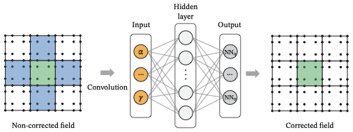
Use structured learned corrections
We study two correction mechanisms: expressive source-term augmentation for compressible DG models and discretization-consistent weak-form corrections for incompressible finite elements.
Why it matters
Improve fidelity without abandoning scientific solvers
The goal is not just better short-horizon fit, but more stable long-time rollouts that remain compatible with existing solvers, adjoints, and conservation constraints.
Motivation
High-fidelity PDE simulations are accurate but expensive. Low-order models are efficient but often miss unresolved dynamics and accumulate rollout error.
This project studies learned correction operators trained end-to-end through differentiable simulators, with the goal of improving long-horizon fidelity while preserving the parts of the numerical method that make scientific simulation trustworthy.
Source term and weak-form correction strategies
The project explores two ways to inject learnable corrections into PDE solvers. They differ in where the correction enters and therefore in the tradeoff between expressivity and numerical consistency.
Source-term correction: expressive forcing for compressible Navier-Stokes (DG)
In the discontinuous Galerkin (DG) setting for the compressible Navier-Stokes equations, we augment the semi-discrete evolution with a learnable source term:
\[ \frac{d\mathbf{u}}{dt} = \mathcal{R}(\mathbf{u}) + \mathcal{S}_{\theta}(\mathbf{u}) \]
Here $\mathbf{u}$ is a state vector of conservative variables (e.g., density, momentum, total energy), $\mathcal{R}(\mathbf{u})$ is the DG discretization of the PDE operator, and $\mathcal{S}_{\theta}(\mathbf{u})$ is a neural source term trained from data (typically from filtered/projected high-fidelity trajectories).
Advantage (expressivity). A source term can represent a wide class of unresolved effects because it is not restricted to a specific discretization component. This is useful when the missing physics acts like an effective closure/parameterization.
Limitation (consistency). A naive additive source can violate discrete invariants. In particular, if the density source has nonzero mean on elements, it can act as an artificial sink/source of mass, and long-horizon rollouts may destabilize. To improve stability, we also study mass-conserving source constructions that enforce an elementwise zero-mean constraint (e.g., zeroing the constant modal coefficient of the density source so that the density source integrates to zero on each element).
Weak-form correction: discretization-consistent operator modifications for incompressible Navier-Stokes (finite elements)
For the incompressible Navier-Stokes equations in a finite element framework, we use a different mechanism: rather than adding a pointwise forcing term, we modify the variational form (i.e., the discrete operator itself). A representative baseline weak form is:
\[ \left(\partial_t \mathbf{u}_h, \mathbf{v}_h\right) + \nu \left(\nabla \mathbf{u}_h, \nabla \mathbf{v}_h\right) + c_{\mathrm{skew}}\left(\mathbf{u}_{\mathrm{adv}};\mathbf{u}_h,\mathbf{v}_h\right) - \left(p_h,\nabla\cdot \mathbf{v}_h\right) + \left(q_h,\nabla\cdot \mathbf{u}_h\right) = 0 \]
and a weak-form-corrected variant augments existing terms through learned coefficient fields, e.g.:
\[ \left(\partial_t \mathbf{u}_h, \mathbf{v}_h\right) + \left((\nu + \nu_t)\nabla \mathbf{u}_h, \nabla \mathbf{v}_h\right) + \left(1 + c_{\mathrm{adv}}\right)c_{\mathrm{skew}}\left(\mathbf{u}_{\mathrm{adv}};\mathbf{u}_h,\mathbf{v}_h\right) + \left(\gamma\,\nabla\cdot \mathbf{u}_h, \nabla\cdot \mathbf{v}_h\right) - \left(p_h,\nabla\cdot \mathbf{v}_h\right) + \left(q_h,\nabla\cdot \mathbf{u}_h\right) = 0 \]
The fields $c_{\mathrm{adv}}(u_h)$, $\nu_t(u_h)$, and $\gamma(u_h)$ are predicted from the coarse solution (often elementwise with neighborhood context) and are bounded to maintain stability/interpretability (e.g., $\nu_t \ge 0$, $\gamma \ge 0$, and moderate advection scaling).
Advantage (consistency). Because the correction is applied through the same assembled bilinear forms, this approach preserves sparsity/locality, tends to remain compatible with existing linear/nonlinear solvers and preconditioners, and supports adjoint-consistent differentiation.
Limitation (expressivity). Weak-form corrections are intentionally structured: you choose which terms to correct and how. This can reduce the hypothesis space, but can also improve conditioning and long-horizon robustness by preventing the correction from “fighting” the discretization.
In benchmark studies, this structure can translate into better optimization behavior (lower training loss) and improved long-horizon accuracy compared with unconstrained strong-form corrections.
Training and differentiation
Across both correction mechanisms, training typically minimizes rollout mismatch to projected/filter-aligned high-fidelity trajectories:
\[ J(\theta) = \sum_{j=0}^{m-1} \left\lVert \tilde{\mathbf{u}}^{j+1}(\theta) - \mathcal{P}\mathbf{u}_H^{j+1} \right\rVert_2^2 \]
with gradients computed by differentiating through the time integrator (e.g., neural ODE / adjoint methods for DG+source models, and discrete adjoints plus backpropagation for weak-form finite element models).
Representative results
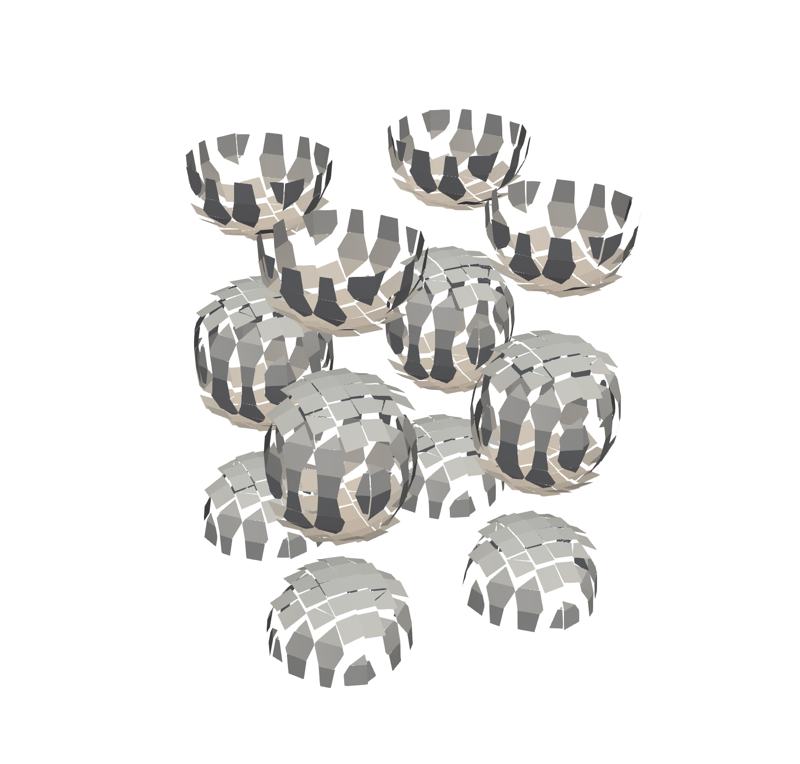
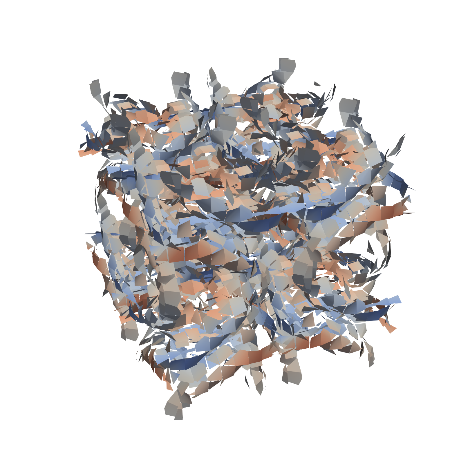
Compressible Navier-Stokes (DG): Q-criterion and conservation
Q-criterion is a standard diagnostic for coherent vortical structures. The examples below illustrate how (i) hybrid corrections can improve coarse-resolution vortical structure and (ii) conservation awareness can matter for long-horizon stability.
Related pages
Funding
- U.S. Department of Energy, Office of Science, Office of Advanced Scientific Computing Research (ASCR) and the Scientific Discovery through Advanced Computing (SciDAC) FASTMath Institute program (FASTMath)
- U.S. Department of Energy, Office of Science, Office of Advanced Scientific Computing Research (ASCR), the Applied Mathematics Program through the Competitive Portfolios Project on Energy Efficient Computing: A Holistic Methodology
- U.S. Department of Energy, Office of Science, Office of Advanced Scientific Computing Research (ASCR) and the Scientific Discovery through Advanced Computing (SciDAC) ASCR-BER partnership program
- Argonne Leadership Computing Facility (ALCF) Postdoctoral Fellowship
References for deeper dive
- Junoh Jung and Emil M Constantinescu. Learning differentiable weak-form corrections to accelerate finite element simulations (proceedings, 2026). arXiv
- Shinhoo Kang and Emil M Constantinescu. Differentiable DG with neural operator source term correction (2025). arXiv
- Shinhoo Kang and Emil M Constantinescu. Learning subgrid-scale models with neural ordinary differential equations. Computers and Fluids, 2023. DOI arXiv