Power Grid and Uncertainty Quantification
This project brings together work on power-grid operations under weather and hazard uncertainty, stochastic models for inverter-based dynamics, adjoint-based sensitivity and inverse methods, and recent surrogate-assisted approaches to security margins and reliability. The common thread is that the grid should be treated as an uncertain dynamical system rather than as a single deterministic operating point.
Scientific question
How should uncertainty enter grid computation?
The work spans scheduling, dynamic simulation, calibration, and security analysis, but the same issue appears in each setting: uncertain inputs must be propagated in a way that is useful for decisions.
Core idea
Combine physics-based models with uncertainty-aware algorithms
The page traces a progression from probabilistic forecast inputs, to stochastic dynamical models, to adjoint-based inference, and finally to calibrated surrogate models for fast security assessment.
What visitors should learn
The right approximation depends on the task
Operations, forecasting, inverse problems, and dynamic security need different tools; the page emphasizes what each tool buys, what it misses, and why later developments became necessary.
Motivation
Modern power systems are shaped by weather, hazard exposure, inverter-based resources, incomplete knowledge of dynamic parameters, and rare but consequential security events. That makes the computational problem broader than classical steady-state analysis. At different stages, one may need to schedule generation under uncertain wind, infer hidden model parameters from transient measurements, propagate stochastic forcing through dynamic simulations, or estimate how close the system is to a critical security boundary. This progression, from weather-aware operations to calibrated security surrogates, is reflected in work ranging from Constantinescu et al. (2011) and Bessa et al. (2012) to Maldonado et al. (2022), Zhao et al. (2024), and Su et al. (2026).
One abstract view is
\[ \min_{u} \ \mathbb{E}\bigl[C(u,\xi)\bigr] \qquad \text{subject to} \qquad g(u,\xi) \le 0, \]
where $u$ collects control decisions and $\xi$ represents uncertain weather, hazard-driven conditions, loads, inverter-based injections, or model parameters. The technical question is not only how to solve such problems, but how to build uncertainty models that remain informative when embedded in large dynamical and optimization workflows.
Weather-aware operations and inverter-based integration
The earliest phase of this line of work focused on bringing weather uncertainty into grid operations in a way that mattered for decisions, not only for forecast verification. That began with reports and conference work in 2009–2010 on exploiting weather forecasts in integrated energy systems and on the economic implications of better forecast information, and it matured into journal work on stochastic unit commitment, probabilistic wind forecasting, and cooling-constrained plant operation. Representative papers in this phase are Constantinescu et al. (2011), Bessa et al. (2012), and Salazar et al. (2013).
In the unit-commitment setting, the key step was to connect ensemble numerical weather prediction to stochastic scheduling. The point was not to generate a single “best” wind forecast, but to pass a scenario-based uncertainty description into commitment and dispatch. That is what makes the 2011 framework important in hindsight: it treats meteorology, forecast uncertainty, and power-system optimization as one pipeline rather than as disconnected tasks (Constantinescu et al., 2011).
The wind-power forecasting work pushed the same lesson further. Conditional kernel density estimation produces full predictive distributions, and the time-adaptive version matters because wind uncertainty is not stationary over the day. Once the output is a density rather than a point, one can ask calibration and sharpness questions that are directly relevant to bidding and reserve decisions (Bessa et al., 2012).
The water-management work adds a different operational constraint: thermal generation is not only limited by fuel and demand, but also by environmental and cooling conditions. That paper shows how stochastic optimization changes the operating point when weather and intake constraints are uncertain, and it broadens the meaning of “energy uncertainty” beyond variable injections alone toward wider hazard-aware operating constraints (Salazar et al., 2013).
The solar-irradiation study is a short but useful bridge in this story. Even though it is not a power-grid dynamics paper, it reinforces the same idea: spatial information and probabilistic prediction are valuable when the end use is operational risk, not just pointwise forecast error (Bilionis et al., 2014).
Advantages and limitations
What improved: these methods moved the workflow from deterministic forecasts to distributions and scenarios that can drive scheduling and bidding decisions.
What remained hard: early operations models still depend heavily on forecast quality, scenario design, and simplified representations of downstream dynamics. They say little by themselves about transient security or parameter uncertainty.
Stochastic uncertainty models for power systems
Once uncertain inverter-based injections are treated as dynamic forcing rather than as exogenous scenarios, the problem becomes one of uncertainty propagation through power-system models, as developed in Wang et al. (2015) and carried into operational flexibility studies such as Li et al. (2016). For a stochastic dynamical system,
\[ d x(t) = f(x(t), z(t))\,dt, \qquad d z(t) = a(z(t))\,dt + B(z(t))\,dW_t, \]
the goal is no longer only to optimize an operating point; it is to understand the evolving distribution of quantities of interest under correlated random input.
The probabilistic density function work addresses exactly this issue (Wang et al., 2015). Instead of relying purely on Monte Carlo sampling, it derives and solves deterministic equations for the probability density associated with stochastic power-system dynamics. That is useful because tail behavior and rare events are often the quantities that matter operationally, and brute-force sampling becomes expensive precisely where the interesting events are rare.
This phase also clarifies a tradeoff that shows up repeatedly later in the project. A reduced probabilistic model can be much more efficient than sampling, but only if the closure assumptions are good enough for the quantity being tracked. Efficiency is not free; it is paid for by modeling assumptions.
The battery-scheduling work is a natural operational extension of this stochastic viewpoint (Li et al., 2016). It shows that uncertainty should not only be forecast, but also converted into flexible operating ranges and recourse decisions. That paper does not replace the PDF-based dynamical viewpoint, but it illustrates how uncertainty quantification becomes operational value only when the control model is allowed to respond to it.
Advantages and limitations
What improved: this stage moved from probabilistic inputs to probabilistic system response, which is the right language for reliability and risk.
What remained hard: reduced stochastic models still need careful closure choices and are not a substitute for scalable inference when the main uncertainty lies in poorly known parameters rather than in exogenous forcing.
Dynamics, sensitivities, and calibration
The next step in the project treats the power grid as a hybrid dynamical system whose behavior depends on control settings, model parameters, switching events, and observation quality, which is the setting addressed by Zhang et al. (2017), Petra et al. (2017), Constantinescu et al. (2020), and Attia et al. (2023). Here the central computational question changes again: if a transient-performance metric depends on many parameters, how can one differentiate, calibrate, and optimize it without paying the cost of one forward simulation per parameter?
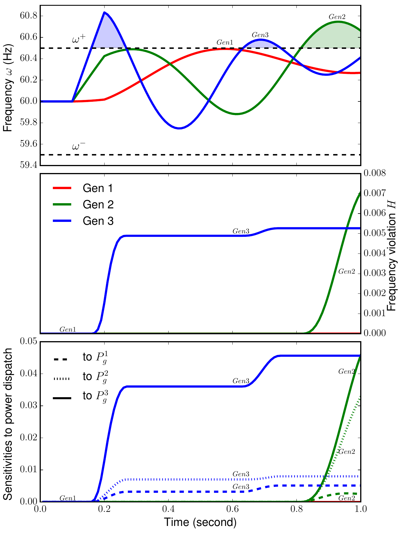
The discrete-adjoint sensitivity work answers that question for hybrid power-system dynamics with switching (Zhang et al., 2017). Its main contribution is not only an adjoint formula, but a consistent treatment of events and jump conditions so that sensitivities remain accurate for the same discrete model that is actually simulated. That consistency is essential once sensitivities are used for optimization rather than only for diagnostics.
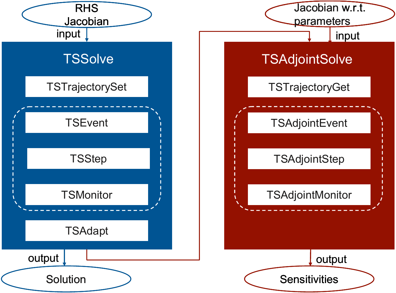
This work also has a software and scalability dimension. The adjoint machinery was implemented in PETSc with checkpointing, event handling, and reusable time-stepping infrastructure, and related work on Krylov–Schwarz solvers addressed the cost of large dynamic simulations themselves (Abhyankar et al., 2017). That combination matters because adjoint methods are only useful in practice if the forward and backward solves scale on realistic systems.
With those ingredients in place, the project moved into dynamic inverse problems. The Bayesian parameter-estimation work targets quantities such as generator inertias that are not observable in steady state and therefore need transient information (Petra et al., 2017). The later statistical-treatment paper generalizes this idea by using proper scoring rules for inverse problems with stochastic forward models, which is a more honest formulation when the forward output is itself a distribution (Constantinescu et al., 2020). The most recent calibration paper pushes further toward centralized variational data assimilation for dynamic models, connecting the inference problem directly to scalable optimization methods (Attia et al., 2023).
Dynamic sensitivities and score-based calibration
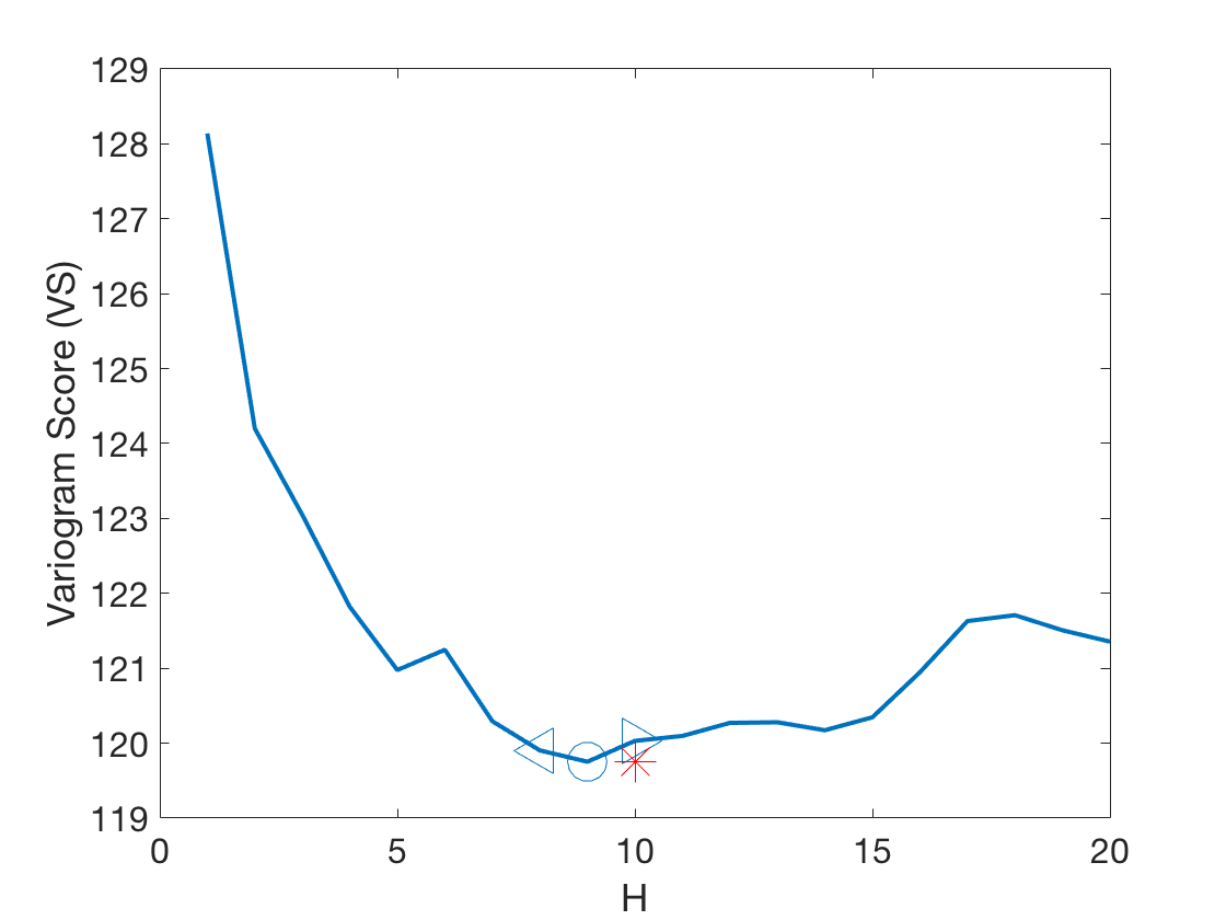
The figures below illustrate the transition from sensitivity analysis to scalable inference: a reusable adjoint workflow, a transient-security sensitivity example on the 9-bus system, and a score-based inverse-identification curve that shows how parameter estimation becomes an optimization problem over uncertainty-aware objectives.
Advantages and limitations
What improved: the work moved from uncertainty propagation alone to gradient-based inference, calibration, and control on realistic dynamic models.
What remained hard: adjoints and variational methods require event-consistent discretizations, scalable solvers, and objectives that remain meaningful when the forward model is stochastic rather than deterministic.
Security margins, extreme trajectories, and surrogate models
Recent work in this area focuses on quantities that are closer to operational security margins: short-time transient amplification, worst-case trajectories over parameter sets, failure probabilities, and load-margin constraints under dynamic line ratings, as developed in Maldonado et al. (2022), Maldonado et al. (2023), Zhao et al. (2024), and Su et al. (2026).
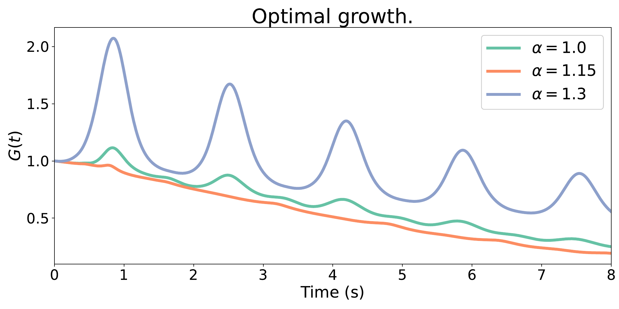
The transient-growth work begins from the observation that eigenvalues alone do not fully characterize short-time dynamic risk (Maldonado et al., 2023). If $\delta x(t)$ is a perturbation to an operating point, the relevant quantity can be written as
\[ G(t) = \max_{\lVert \delta x_0 \rVert = 1} \lVert \delta x(t) \rVert, \]
which captures the largest pre-asymptotic amplification over all admissible initial perturbations. That perspective is useful because inverter-based systems can exhibit significant short-term growth even when asymptotic modal analysis looks benign.
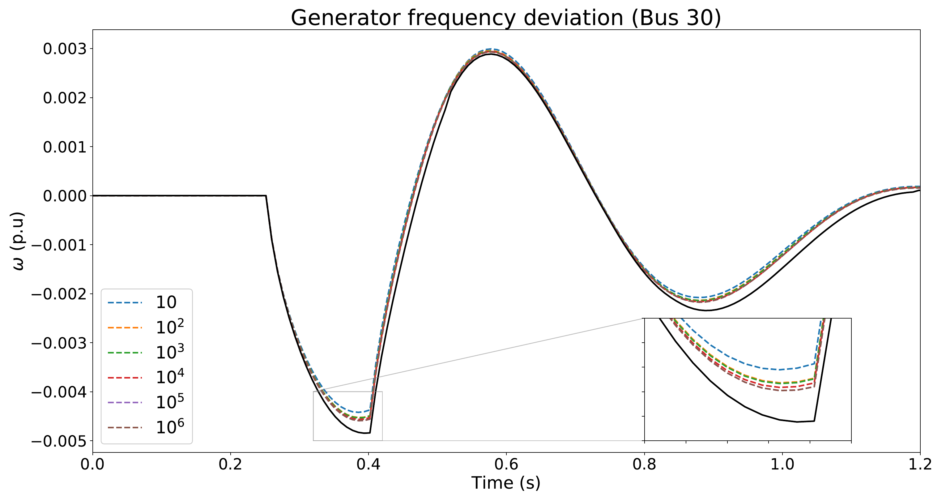
The trust-region trajectory work addresses a related, but nonlinear, question: how can one compute extreme trajectories over uncertain parameter sets without relying on prohibitively large Monte Carlo ensembles (Maldonado et al., 2022). The answer is to combine sensitivity information with a trust-region optimization procedure that keeps the local approximation under control when nonlinear effects become important. This is exactly the kind of place where the page should teach a clear pro/con lesson: local surrogates are powerful, but only if the algorithm monitors when the local model stops being trustworthy.
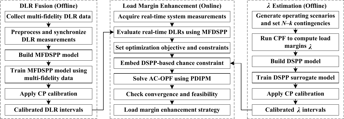
The most recent reliability-oriented papers continue this progression. One estimates failure probabilities in correlated structure-preserving stochastic models, pushing uncertainty quantification closer to tail events that matter operationally (Zhao et al., 2024). The newest work then combines multi-fidelity dynamic line rating, conformal uncertainty calibration, and learned load-margin surrogates in a real-time control setting (Su et al., 2026). The underlying idea is attractive: use data-driven models for speed, but force them to remain tied to physically meaningful security quantities such as line ratings and load margin.
Transient growth and extreme trajectories
The first figure shows why modal stability alone is not enough: the 39-bus system can exhibit substantial short-time amplification as loading increases. The second figure shows the complementary nonlinear question, where a trust-region method approximates the extreme trajectory and is compared against Monte Carlo estimates.
Surrogate-assisted reliability and load-margin enhancement
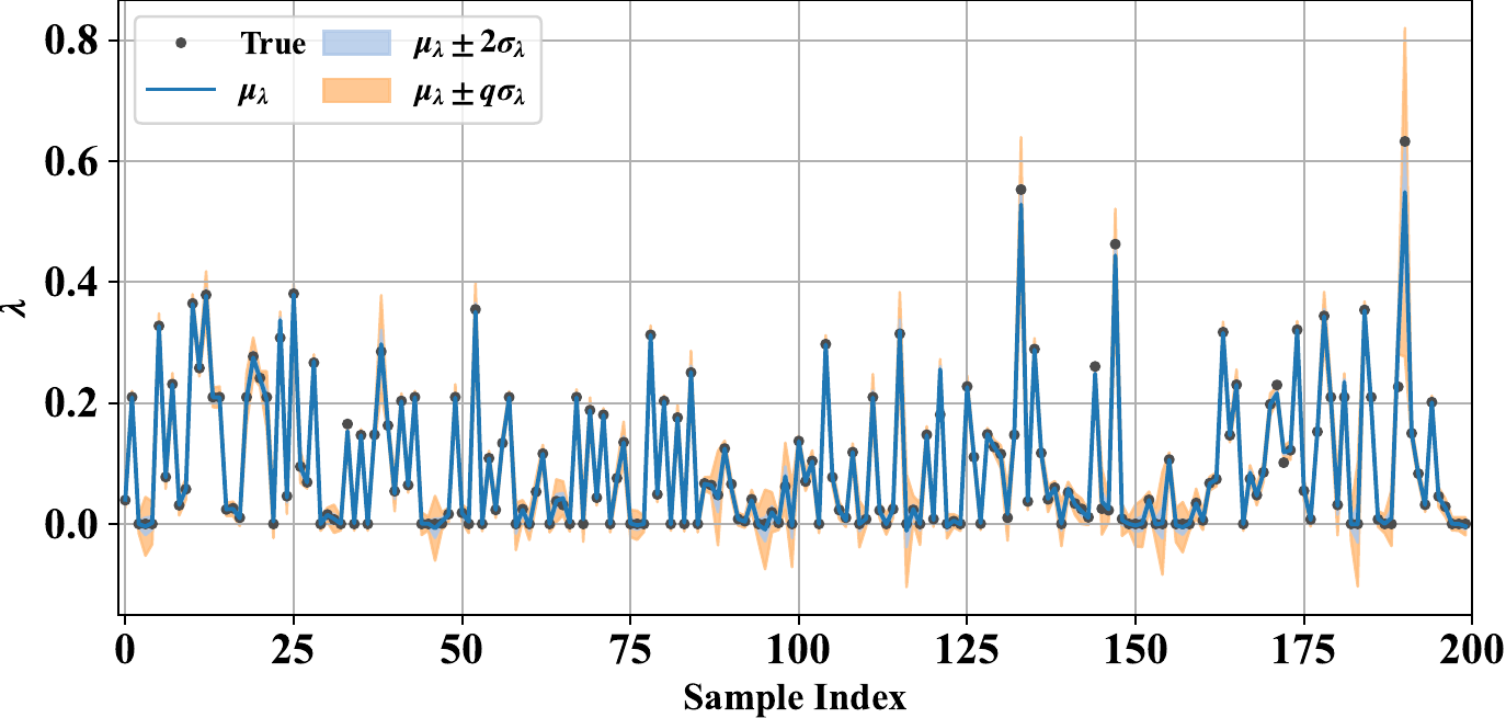
The recent security work uses surrogate models because the underlying continuation-power-flow and stochastic-dynamics calculations are too expensive to repeat online. The diagrams below emphasize that the surrogate is useful only because it is calibrated against physically meaningful quantities and wrapped in uncertainty estimates.
\[ \mathbb{P}\!\left(\lambda \ge \lambda_{\min}\right) \ge 1-\alpha \]
Advantages and limitations
What improved: recent work turns security analysis into quantities that are both operationally meaningful and fast enough to be embedded in decision workflows.
What remains hard: surrogate models only help if their uncertainty is calibrated and their outputs stay tied to physical notions of margin, failure, and feasibility. A fast but uncalibrated surrogate can be more dangerous than an expensive solver.
Lessons learned
Lessons learned
Probabilistic forecasts are more useful than point forecasts for decisions. Once the task is commitment, bidding, or reserve management, distributions and scenarios matter more than a single best guess.
Dynamic security is not an eigenvalue-only problem. Short-time amplification, switching events, and nonlinear trajectory extremes can dominate the behavior that matters operationally.
Adjoints and scalable solvers become essential as soon as inference enters the loop. Calibration and dynamic optimization are not practical without reusable sensitivity infrastructure and parallel forward/backward solves.
Data-driven surrogates are valuable only when they remain tied to physics-based margins. The strongest recent results use learned models for speed, but keep security quantities such as line ratings, load margins, and calibrated uncertainty intervals at the center.
Funding
- U.S. Department of Energy, Office of Science, Office of Advanced Scientific Computing Research (ASCR) and the Scientific Discovery through Advanced Computing (SciDAC) FASTMath Institute program (FASTMath), and the SciDAC ASCR-OE (Office of Electricity) partnership.
- U.S. Department of Energy, Office of Science, Office of Advanced Scientific Computing Research (ASCR), the Applied Mathematics Program through the Competitive Portfolios Project on Energy Efficient Computing: A Holistic Methodology.
Related pages
References
Weather-aware operations and inverter-based integration
- Emil M Constantinescu,Victor Zavala, Matthew Rocklin, Sangmin Lee, and Mihai Anitescu. A computational framework for uncertainty quantification and stochastic optimization in unit commitment with wind power generation. IEEE Transactions on Power Systems, Vol. 26(1); Pages 431-441, 2011. [DOI]
- Ricardo J. Bessa, Vladimiro Miranda, Audun Botterud, Jianhui Wang, and Emil M Constantinescu. Time adaptive conditional kernel density estimation for wind power forecasting. IEEE Transactions on Sustainable Energy (Special Wind Energy issue), Vol. 3(4); Pages 660-669, 2012. [DOI]
- Juan M. Salazar, Urmila Diwekar, Emil M Constantinescu, and Victor Zavala. Stochastic optimization approach to water management in cooling-constrained power plants. Applied Energy, Vol. 112; Pages 12-22, 2013. [DOI]
Stochastic uncertainty models
- Peng Wang, David Barajas-Solano, Emil M Constantinescu, Shrirang S. Abhyankar, Debojyoti Ghosh, Barry Smith, Zhenyu Huang, and Alexandre Tartakovsky. Probabilistic density function method for stochastic ODEs of power systems with uncertain power input. SIAM/ASA Journal on Uncertainty Quantification (JUQ), Vol. 3(1); Pages 873-896, 2015. [DOI]
Dynamics, sensitivities, and calibration
- Hong Zhang, Shrirang S. Abhyankar, Emil M Constantinescu, and Mihai Anitescu. Discrete adjoint sensitivity analysis of power system dynamics. {"IEEE Transactions on Circuits and Systems--I"=>"Regular Papers"}, Vol. 64(5); Pages 1247-1259, 2017. [DOI]
- Noemi Petra, Cosmin G. Petra, Zheng Zhang, Emil M Constantinescu, and Mihai Anitescu. A Bayesian approach for parameter estimation with uncertainty for dynamic power systems. IEEE Transactions on Power Systems, Vol. 32(4); Pages 2735-2743, 2017. [DOI] [arXiv]
- Emil M Constantinescu, Noemi Petra, Julie Bessac, and Cosmin G. Petra. Statistical treatment of inverse problems constrained by differential equations-based models with stochastic terms. SIAM Journal on Uncertainty Quantification, Vol. 8(1); Pages 170-197, 2020. [DOI] [arXiv]
- Ahmed Attia, D. Adrian Maldonado, Emil M Constantinescu, and Mihai Anitescu. Centralized calibration of power system dynamic models using variational data assimilation. 2023. [arXiv] [PDF]
Security margins, reliability, and surrogate models
- Adrian Maldonado, Emil M Constantinescu, Hong Zhang, Vishwas Rao, and Mihai Anitescu. Trust-region approximation of extreme trajectories in power system dynamics. IEEE Transactions on Power Systems, Vol. 37(5); Pages 3937-3946, 2022. [DOI] [arXiv]
- Daniel Adrian Maldonado, Emil M Constantinescu, Junbo Zhao, and Mihai Anitescu. Computationally efficient power system maximum transient linear growth estimation. Submitted, 2023. [arXiv] [PDF]
- Hongli Zhao, Tyler E. Maltba, D. Adrian Maldonado, Emil M Constantinescu, and Mihai Anitescu. Data-driven estimation of failure probabilities in correlated structure-preserving stochastic power system models. 2024. [arXiv]
- Tong Su, Junbo Zhao, Emil M Constantinescu, and Cosmin G. Petra. Multi-fidelity dynamic line rating fusion for system load margin enhancement with large-scale offshore wind generations. IEEE Transactions on Power Systems, Pages 1-14, 2026. [DOI]