Time Integration Project: Robust time stepping for stiff and multiscale PDEs
This project develops time integration algorithms for stiff and multiscale dynamical systems arising from PDE discretizations. The focus is on methods that remain accurate in long simulations while scaling to large problems: strong-stability-preserving (SSP) schemes, general linear methods (GLMs), implicit-explicit (IMEX) integration, multirate time stepping, and global error estimation.
Scientific question
How should time integrators adapt to stiff, multiscale dynamics?
After spatial discretization, many PDEs become very large ODE or DAE systems whose fastest scales can dominate stability, cost, and accumulated error.
Core idea
Exploit structure instead of brute force
The methods here use SSP design, implicit-explicit splitting, multirate partitions, and explicit global-error tracking to target the right source of difficulty in each problem.
Practical outcome
Algorithms that land in production software
A key objective is not just analysis, but methods that can be implemented in libraries such as PETSc TS and DESolve for real scientific simulation workflows.
Motivation
Many scientific applications evolve PDEs in time. After spatial discretization, these problems typically take the form of large ODE systems:
\[ \frac{d u_h(t)}{dt} = F_h(u_h(t), t), \qquad u_h(0) = u_{h,0}. \]
Two challenges tend to dominate:
- Stiffness: fast physics or fine spatial scales can force prohibitively small explicit time steps.
- Multiple time scales: different components (or spatial regions) evolve at very different rates.
This project explores integrators that exploit structure (splittings, partitions, and error estimators) to improve efficiency while maintaining stability and reliable accuracy.
Topic 1: New methodologies for numerical integrators
At the core are one-step (Runge-Kutta) and multistep (linear multistep) methods. For hyperbolic PDEs and nonlinear conservation laws, robustness often means preserving stability properties that are known to hold under forward Euler, such as monotonicity or total-variation-diminishing (TVD) behavior.
Strong stability preserving (SSP) time stepping
An SSP method is designed so that, under an appropriate step-size restriction, it can be expressed as a convex combination of forward Euler updates. This provides a principled way to build higher-order methods that inherit nonlinear stability properties important in PDE simulations.
General linear methods (GLMs)
GLMs unify Runge-Kutta and linear multistep methods within a single framework. A compact representation is:
\[ Y = h A F(Y) + U\,y^{[n-1]}, \qquad y^{[n]} = h B F(Y) + V\,y^{[n-1]}, \]
where $Y$ collects stage values, $y^{[n]}$ stores the propagated solution history, and $(A,B,U,V)$ define the method. This view is useful for designing schemes with properties that matter in PDE settings, such as high stage order (to mitigate order reduction in stiff problems) and SSP behavior. GLMs also provide a natural bridge to linearly implicit (Rosenbrock-type) constructions and to methods with embedded error estimation.
Advantages and limitations
Advantages: principled stability design (SSP) and a unified design space (GLMs) that can improve long-time robustness for PDE discretizations.
Limitations: higher-order SSP/GLM designs can increase stage count or coupling complexity, and practical performance depends on implementation details (e.g., Jacobian reuse, preconditioning, and adaptivity).
Selected references
- Emil M Constantinescu and Adrian Sandu. Optimal strong-stability-preserving general linear methods. SIAM Journal on Scientific Computing (SISC), Vol. 32(5); Pages 3130-3150, 2010. [DOI]
- Emil M Constantinescu. On the order of general linear methods. Applied Mathematics Letters, Vol. 22(9); Pages 1425-1428, 2009. [DOI]
Topic 2: Implicit-explicit (IMEX) and splitting methods
In many PDE models, different terms have very different stiffness and solver cost. IMEX methods start from an additive split
\[ F_h(u,t) = F_E(u,t) + F_I(u,t), \]
where $F_E$ is treated explicitly (cheap, nonstiff) and $F_I$ is treated implicitly (stiff, but often structured so that robust solvers and preconditioners apply). IMEX is particularly attractive for multiphysics coupling and for systems where a fully implicit method would be too expensive.
When IMEX works best
Best use cases: a clean split with a stiff component that is well-handled by scalable implicit solvers, and a nonstiff component that would otherwise enforce small explicit steps.
Typical limitations: splitting error and nonlinear coupling can reduce effective order (order reduction), and stability constraints may still depend on the explicit component or on how the split is defined.
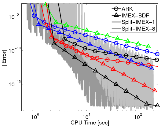
Accuracy and cost tradeoffs in IMEX designs
IMEX design is ultimately about balancing stability and accuracy against solver cost. This figure shows a representative cost-versus-error comparison across different IMEX-type strategies.
Selected references
- Emil M Constantinescu and Adrian Sandu. Extrapolated implicit-explicit time stepping. SIAM Journal on Scientific Computing (SISC), Vol. 31(6); Pages 4452-4477, 2010. [DOI]
- Daniel S. Abdi, Francis X. Giraldo, Emil M. Constantinescu, Lester E. Carr III, Lucas C. Wilcox, and Timothy Warburton. Acceleration of an implicit-explicit non-hydrostatic unified model of the atmospheric (NUMA) on manycore processors. International Journal of High Performance Computing Applications, Vol. 33(2); Pages 242-267, 2019. [DOI] [arXiv] [PDF]
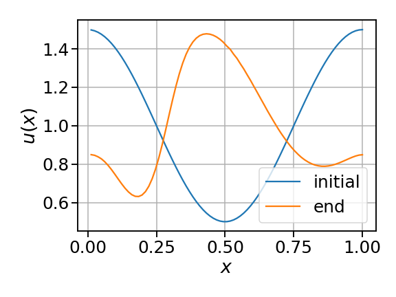
Topic 3: Multirate methods for multiple time scales
Multirate methods target problems where some components evolve fast and others evolve slowly. One way to express this is a partition:
\[ \frac{d u}{dt} = f_{\mathrm{slow}}(u,t) + f_{\mathrm{fast}}(u,t). \]
The goal is to take a large macro step for the slow dynamics while resolving the fast dynamics with cheaper micro steps, often only where needed (e.g., localized fast regions in space).
This project studies multirate methods built from several design patterns:
- Multirate Runge-Kutta (MRK): RK stages are coupled across fast/slow components with controlled information exchange.
- Multirate linear multistep (MR-LMM): multistep history is advanced with different step sizes for different components.
- Multirate extrapolation: a hierarchy of solves at different resolutions is combined by extrapolation to improve accuracy without fully resolving all components at the smallest step size.
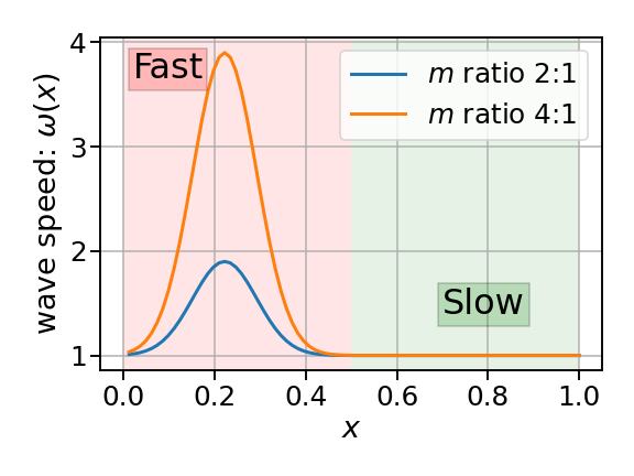
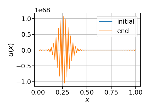
Fast and slow regions, coupling, and stability
The central multirate question is how to couple fast and slow updates so that the combined method is stable and accurate. The figures below illustrate fast/slow structure, error behavior, and the impact of coupling choices on stability.
Advantages and limitations
Advantages: reduces cost by resolving fast dynamics only as needed while taking large steps for slow dynamics.
Limitations: stability and accuracy depend on coupling design; fast/slow partitions that change in time or space require careful treatment to avoid drift or instability.
Selected references
- Emil M Constantinescu and Adrian Sandu. Multirate timestepping methods for hyperbolic conservation laws. Journal of Scientific Computing, Vol. 33(3); Pages 239-278, 2007. [DOI] [PDF]
- Adrian Sandu and Emil M Constantinescu. Multirate explicit Adams methods for time integration of conservation laws. Journal of Scientific Computing, Vol. 38(2); Pages 229-249, 2009. [DOI] [PDF]
- Emil M Constantinescu and Adrian Sandu. On multirate numerical integration methods. (invited) The European Consortium for Mathematics in Industry (ECMI-2008) in Progress in Industrial Mathematics at ECMI 2008, University College London, England, June 30 - July 4, 2008, Vol. 15(2); Pages 341-347, 2010. [DOI]
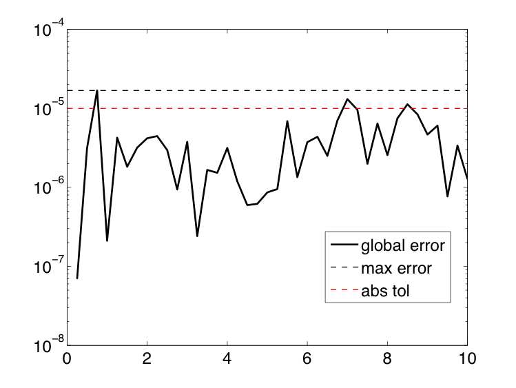
Topic 4: Global error estimation and control
Most adaptive time integrators choose the time step by controlling a local error estimate (LEE), for example from an embedded method pair. This is effective for short integrations, but it does not directly control the global error $e^{[n]} = y^{[n]} - y(t_n)$, which can drift above tolerance over long horizons or in problems with unstable components.
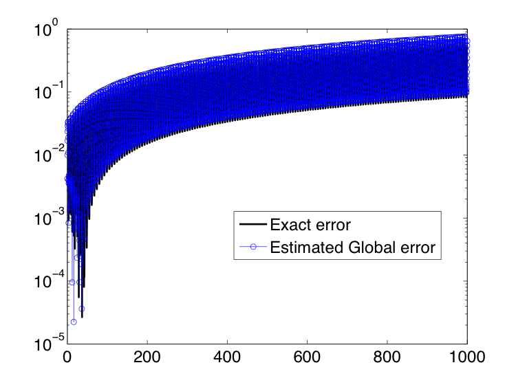
Global error estimation methods augment the integrator so that an estimate of the accumulated error is propagated alongside the solution. In the approach developed in this project, a general linear method evolves both the numerical solution $y^{[n]}$ and an error estimate $\varepsilon^{[n]}$:
\[ \{y^{[n]},\varepsilon^{[n]}\} = \mathcal{G}_h(\{y^{[n-1]},\varepsilon^{[n-1]}\}), \qquad \widehat{y}^{[n]} = y^{[n]} + \varepsilon^{[n]}, \qquad \varepsilon_{\mathrm{loc}}^{[n]} = \varepsilon^{[n]} - \varepsilon^{[n-1]}. \]
Advantage. The estimator targets the quantity of interest (global error) rather than an indirect proxy, which is better suited for long-time integration and for detecting when local-error-controlled simulations silently accumulate unacceptable error.
Limitation. As with any estimator, accuracy depends on the problem class and method design; global-error-aware adaptivity introduces additional parameters and requires careful stability analysis.
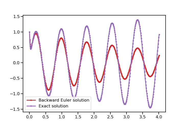
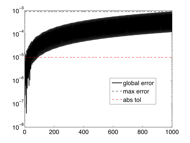
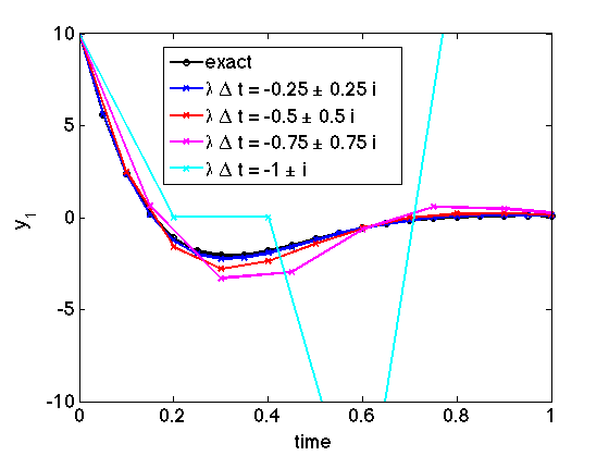
Local versus global error behavior
Local error control can appear successful on short windows while the accumulated global error grows over long horizons. Global error estimation explicitly tracks the accumulated error and can remain informative in long-time simulations.
Selected references
- Emil M Constantinescu. Generalizing global error estimation for ordinary differential equations by using coupled time-stepping methods. Journal of Computational and Applied Mathematics, Vol. 332(C); Pages 140-158, 2018. [DOI] [arXiv]
Software
Many of the methods above are available in open-source libraries used in production simulations.
PETSc TS
HPC time stepping
Includes ARKIMEX, global error estimation methods (GLEE), and multirate time stepping for large-scale ODE/DAE systems.
DESolve
Time integration package
Research implementation of MREXIM, along with prototyping of stiff and multirate integrators.
Related pages
Funding
- U.S. Department of Energy, Office of Science, Office of Advanced Scientific Computing Research (ASCR), the Applied Mathematics Program.
- U.S. National Science Foundation (on earlier work, prior to 2008)
References for deeper dive
The references below are selected to match the four method families highlighted on this page.
- Emil M Constantinescu and Adrian Sandu. Optimal strong-stability-preserving general linear methods. SIAM Journal on Scientific Computing (SISC), Vol. 32(5); Pages 3130-3150, 2010. [DOI]
- Emil M Constantinescu and Adrian Sandu. Extrapolated implicit-explicit time stepping. SIAM Journal on Scientific Computing (SISC), Vol. 31(6); Pages 4452-4477, 2010. [DOI]
- Adrian Sandu and Emil M Constantinescu. Multirate explicit Adams methods for time integration of conservation laws. Journal of Scientific Computing, Vol. 38(2); Pages 229-249, 2009. [DOI] [PDF]
- Emil M Constantinescu. Generalizing global error estimation for ordinary differential equations by using coupled time-stepping methods. Journal of Computational and Applied Mathematics, Vol. 332(C); Pages 140-158, 2018. [DOI] [arXiv]